
close
Choose Your Site
Global
Social Media

Views: 0 Author: Site Editor Publish Time: 2026-09-17 Origin: Site


The mechanical reliability of interconnects dictates whether a larger system thrives or fails. Arbitrary force limits create massive blind spots for manufacturing teams. They lead to dual risks. High false-rejection rates frustrate quality assurance operators. Conversely, loose tolerances cause premature field failures. These failures often stem from fretting wear and poor mating connections.
Engineers need objective data to establish proper specifications. This guide breaks down how to build data-backed thresholds. We will explore international testing standards and application realities. You will understand criteria for evaluating equipment accuracy.
Optimizing these processes reduces friction on the assembly line. It ensures end-user satisfaction. You will learn how to transition from generic supplier guidelines to tailored process controls. We will show you how precision hardware shapes production outcomes.
Effective test limits must balance theoretical industry standards (e.g., EIA, ISO) with application-specific environmental realities.
The accuracy of a connector insertion force testing protocol relies heavily on load cell resolution, axial alignment, and controlled test speeds.
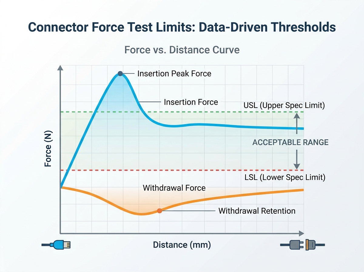
Selecting a plug-in force tester requires evaluating data acquisition rates and software capable of plotting force-vs-distance curves, not just peak force.
Statistical Process Control (SPC) and empirical sample testing are mandatory for setting viable Upper and Lower Spec Limits (USL/LSL).
Miscalibration drains corporate resources rapidly. Over-engineered limits generate excessive scrap. They cause immediate manufacturing bottlenecks. QA teams reject perfectly viable parts. Conversely, under-engineered limits introduce severe field risks. They cause intermittent signal loss. They frustrate end-users during final product assembly.
Insertion force measures the peak effort required to mate two halves. The connector withdrawal force test measures retention reliability. These dynamics require asymmetrical limit setting. Terminal designs dictate these specific curves. Plating materials also alter friction dynamics heavily. You cannot use symmetrical limits for both directions.
Define your success criteria early. You might be validating a newly designed terminal. You might be running routine batch QA. You could be auditing an external supplier. Your specific goals shape the required testing parameters.
Baseline limits often originate from established frameworks. Documents like EIA-364-13 and ISO 20076 govern fundamental procedures. They standardize test speed and sample preparation. They dictate strict environmental conditions. These frameworks give global engineers a common reference point.
However, passing an ISO standard rarely guarantees field success. We call this discrepancy the compliance gap. Real-world applications face harsh physical conditions. Blind mating scenarios introduce awkward angles. High-vibration environments demand tighter retention. Thermal expansion shifts mechanical tolerances. Generic standards cannot predict these variables.
You must establish tailored tolerance bands. Move away from generic supplier datasheets. Leverage historical failure data to inform your decisions. Add sensible safety margins based on field returns. This tailored approach builds a robust testing environment.
Test speed drastically alters recorded measurements. Velocity directly impacts the coefficient of friction. Fast feed rates distort peak force readings artificially. Kinetic friction differs entirely from static friction. You must standardize your mm/min rates strictly across all batches.
Axial alignment presents constant engineering challenges. Off-axis loading ruins data integrity immediately. Improper fixturing introduces parasitic friction into the system. This parasitic drag produces false-high readings. Accurate data demands perfect centerline alignment during every stroke.
Wear degrades components steadily over time. You must factor the degradation curve into your limits. Initial mating forces differ from later cycles. Limits must account for the first mating cycle. They must also account for the 500th cycle depending on product lifespan. Gold plating wears differently than tin.
Resolution separates adequate testers from excellent instruments. Standard tension testers lack specialized micro-accuracy. Load cell sizing must perfectly match the expected force range. This sizing maintains error margins below 0.5 percent. Oversized load cells fail to register subtle friction spikes.
Data Acquisition (DAQ) rates hold immense importance. Capturing a single peak force number is insufficient. You need a continuous, high-resolution curve. This force-versus-distance plot identifies transient binding issues. High DAQ rates catch momentary snags during pin engagement.
Assess frame stiffness thoroughly before procurement. The machine must resist flexing under load. You need self-aligning floating fixtures. They prevent angular misalignment naturally. A rigid frame ensures the sensor measures only the connector.
Software must handle Statistical Process Control seamlessly. It should automatically calculate Cpk for production runs. The software must overlay historical curves for visual comparison. It should export compliance reports directly into factory QMS systems.
Feature Category | Standard UTM Testing Machine | Dedicated Interconnect Tester |
|---|---|---|
Data Plotting | Basic peak force capture | Continuous Force-Distance mapping |
Fixturing | Fixed rigid grips | Self-aligning floating fixtures |
Load Cell Sizing | Often oversized (10kN+) | Micro-scaled for low force (50N - 500N) |
DAQ Rate | Low frequency (50 Hz) | High frequency (1000+ Hz) |
Setting test limits requires methodical statistical validation. You cannot guess these numbers. We recommend a three-phase approach to build a resilient specification framework.
Phase 1: Baseline Profiling
Run a statistically significant sample size first. Test thirty to fifty units of known-good assemblies. This exercise establishes a natural process variation baseline. It shows you how parts behave under ideal manufacturing conditions. You build a normal distribution curve from this initial data.
Phase 2: Defining USL and LSL
Apply a standard deviation multiplier to your baseline data. Six Sigma practices recommend specific mathematical boundaries. Set the Upper Specification Limit to maintain an ergonomic threshold. Set the Lower Specification Limit to ensure retention reliability. The gap between them represents your manufacturing tolerance.
Parameter | Calculation Method | Primary Engineering Goal |
|---|---|---|
USL (Upper Limit) | Mean + (3 × Standard Deviation) | Prevent user fatigue and terminal crushing |
Nominal Target | Baseline Mean Average | Ideal standard performance |
LSL (Lower Limit) | Mean - (3 × Standard Deviation) | Ensure electrical contact and retention |
Phase 3: Gauge R&R (Repeatability and Reproducibility)
Prove your equipment yields consistent data before proceeding. Operators must test multiple parts across multiple trials. You must prove the measurement system itself adds minimal variance. Lock in your final limits only after achieving passing Gauge R&R scores.
Clean all sample parts to remove transient debris.
Condition samples in standard temperature and humidity environments.
Execute baseline profiling runs using floating fixtures.
Calculate historical standard deviations.
Set preliminary USL and LSL values.
Run a formal Gauge R&R study across three operators.
Lock limit parameters in the testing software.
In-house testing equipment serves high-volume production best. It allows rapid prototyping iteration for design teams. It offers strict intellectual property control. However, this route requires upfront CapEx investment. You must also maintain strict internal calibration protocols annually.
Third-party lab services suit different business models. They work perfectly for infrequent batch auditing. They provide independent verification for ISO certification requirements. They also excel at one-off failure analysis. Labs offer objective third-party data without hardware maintenance overhead.
Structure your procurement process carefully. Write a detailed Request for Proposal (RFP). Request physical demo tests using your specific connector samples. Evaluate how easily the software overlays complex curves. Validate equipment alignment usability prior to issuing a purchase order.
Setting proper limits is a deeply empirical process. It never relies on simple guesswork. It requires a synthesis of standard compliance and statistical analysis. Precision equipment acts as the foundation for reliable data.
Standard compliance provides a baseline, but application realities require custom adjustments.
Data plotting reveals hidden friction anomalies far better than peak force numbers.
Statistical process control prevents unnecessary scrap and field failures.
Take actionable steps today to improve your quality control. Encourage evaluators to review their current fixture alignment immediately. Audit your historical force-curve data for hidden trends. Request a technical consultation or a sample test from a reputable equipment manufacturer.
A: The EIA-364-13 standard typically mandates a speed of 25.4 mm/min (1 inch per minute). Deviation alters the kinetic friction coefficient. Faster speeds often create artificial force spikes. Slower speeds fail to simulate real-world human insertion dynamics accurately.
A: Mating cycles erode thin plating materials like gold or tin. This erosion exposes underplates. The coefficient of friction changes drastically as surfaces roughen. Withdrawal forces often increase or become erratic after 100 cycles due to this mechanical degradation.
A: Standard UTMs are highly versatile but often lack specialized interconnect capabilities. They typically lack self-aligning floating fixtures. They also struggle with rapid force-drop detection required for small form-factor parts. Dedicated testers provide higher resolution for micro-friction analysis.


